google-styleguide - Project Hosting on Google Code

google-styleguide - Project Hosting on Google Code

InfoQ: Devs Are From Mars. SETs Are Too.

InfoQ: Devs Are From Mars. SETs Are Too.

Understanding Cassandra Code Base | PrettyPrint.me

Understanding Cassandra Code Base | PrettyPrint.me

Understanding Cassandra Code Base

Lately I’ve been adding some random small features to cassandra so I took the time to have a closer look at the internal design of the system.
While with some features added, such as an embedded service, I could have certainly get away without good understanding of the codebase and design, others, such as the truncate feature require good understanding of the various algorithms used, such as how writes are performed, how reads are performed, how values are deleted (hint: they are not…) etc.

The codebase, although isn’t very large, about 91136 lines, is quite dense and packed with algorithmic sauce, so simply reading through it just didn’t cut it for me. (I used the following kong-fu to count: $ cassandra/trunk $ find * -name *.java -type f -exec cat {} \;|wc -l)

I’m writing this post in hope it’d help others get up to speed. I’m not going to cover the basics, such as what is cassandra, how to deploy, how to checkout code, how to build, how to download thrift etc. I’m also not going to cover the real algorithmic complicated parts, such as how merkle trees are used by the ae-service, how bloom filters are used in different parts of cassandra (and what are they), how gossip is used etc. I don’t think I’m the right person to explain all this, plus there are already bits of those in the cassandra developer wiki. What I am going to write about is what was the path that I took in order to learn cassandra and what I’ve learned along the way. I haven’t found all that stuff documented somewhere else (perhaps I’ll contribute it back to the wiki when I’m done) so I think I’d be very helpful to have it next time I dive into a new codebase.

Lastly, a disclaimer: The views expressed here are simply my personal understanding of how the system works, they are both incomplete and inaccurate, so be warned. Keep in mind that I’m only learning and still sort of new to cassandra. Please also keep in mind that cassandra is a moving target and keeps changing so rapidly that any given snapshot of the code will get irrelevant sooner or later. By the time of writing this the currently official version is 0.6.1 but I’m working on trunk towards 0.7.0.

Here’s a description of the steps I took and things I learned.

Download, configure, run…

First you need to download the code and run unit tests. If you use eclipse, idea, netbeans, vi, emacs and what not, you want to configure it. That was easy. There’s more here.

Reading

Next you want to read some of the background material, depending on what part exactly you want to work on. I wanted to understand the read path, write path and how values are deleted, so I read the following documents about 5 times each. Yes, 5 times. Each. They are packed with information and I found myself absorbing a few more details each time I read. I used to read the document, get back to the source code, make sure I understand how the algorithm maps to the methods and classes, reread the document, reread the source code, read the unit tests (and run them, with a debugger) etc. Here are the docs.

http://wiki.apache.org/cassandra/ArchitectureInternals

SEDA paper

http://wiki.apache.org/cassandra/HintedHandoff

http://wiki.apache.org/cassandra/ArchitectureAntiEntropy

http://wiki.apache.org/cassandra/ArchitectureSSTable

http://wiki.apache.org/cassandra/ArchitectureCommitLog

http://wiki.apache.org/cassandra/DistributedDeletes

I also read the google BigTable paper and the fascinating Amazon’s Dynamo paper, but that was a long time ago. They are good as background material, but not required to understand actual bits of code.

Well, after having read all this I was starting to get a clue what can be done and how but I still didn’t feel I’m at the level of really coding new features. After reading through the code a few times I realized I’m kind of stuck and still don’t understand things like “how do values really get deleted”, which class is responsible for which functionality, what stages are there and how is data flowing between stages, or “how can I mark and entire column family as deleted”, which is what I really wanted to do with the truncate operation.

Stages

Cassandra operates in a concurrency model described by the SEDA paper. This basically means that, unlike many other concurrent systems, an operation, say a write operation, does not start and end by the same thread. Instead, an operation starts at one thread, which then passes it to another thread (asynchronously), which then passes it to another thread etc, until it ends. As a matter of fact, the operation doesn’t exactly flow b/w threads, it actually flows b/w stages. It moves from one stage to another. Each stage is associated with a thread pool and this thread pool executes the operation when it’s convenient to it. Some operations are IO bound, some are disk or network bound, so “convenience” is determined by resource availability. The SEDA paper explains this process very well (good read, worth your time), but basically what you gain by that is higher level of concurrently and better resource management, resource being CPU, disk, network etc.

So, to understand data flow in cassandra you first need to understand SEDA. Then you need to know which stages exist in cassandra and exactly does the data flow b/w them.

Fortunately, to get you started, a partial list of stages is present at the StageManager class:

public final static String READ_STAGE = "ROW-READ-STAGE";
public final static String MUTATION_STAGE = "ROW-MUTATION-STAGE";
public final static String STREAM_STAGE = "STREAM-STAGE";
public final static String GOSSIP_STAGE = "GS";
public static final String RESPONSE_STAGE = "RESPONSE-STAGE";
public final static String AE_SERVICE_STAGE = "AE-SERVICE-STAGE";
private static final String LOADBALANCE_STAGE = "LOAD-BALANCER-STAGE";

I won’t go into detail about what each and every stage is responsible for (b/c I don’t know…) but I can say that, in short, we have the ROW-READ-STAGE which takes part in the read operation, the ROW-MUTATION-STAGE which takes part in the write and delete operations, the AE-SERVICE-STAGE which is responsible for anti-entropy. This is not a comprehensive list of stages, depending on the code path you’re interested in, you may find more along the way. For example, browsing the file ColumnFamilyStore you’ll find some more stages, such as FLUSH-SORTER-POOL, FLUSH-WRITER-POOL and MEMTABLE-POST-FLUSHER. In Cassandra stages are identified by instances of the ExecutorService, which is more or less a thread pool and they all have all-caps names, such as MEMTABLE-POST-FLUSHER.

To visualize that I created a diagram that mixes both classes and stages. This isn’t valid UML, but I think it’s a good way to look at how data flows in the system. This is not a comprehensive diagram of all classes and all stages, just the ones that were interesting to me.

yUML source

Debugging

Reading through the code using a debugger, while running a unit-test is an awesome way to get things into your head. I’m not a huge fan of debuggers, but one thing they are good at is learning a new codebase by singlestepping into unit tests. So what I did was to run the unit-tests while single stepping into the code. That was awesome. I also ran the unit tests for Hector, which uses the thrift interface and spawn an embedded cassandra server so they were right to the point, user friendly and eye opening.

Class Diagrams

Next thing I did is use a tool to extract class diagrams from the existing codebase. That was not a great use of my time.

Well, the tool I used wasn’t great, but that’s not the point. The point is that cassandra’s codebase is written in such way that class diagrams help very little in understanding it. UML class diagrams are great for object oriented design. The essence of them is the list of classes, class members and their relationships. For example if a class A has a list of Bs, so you can draw that in a UML class diagram such that A is an aggregation of Bs and just by looking at the diagram you learn a lot. For example, an Airplane has a list of Passengers.

Cassandra is a complex system with solid algorithmic background and excellent performance, but, to be honest, IMO from the sole perspective of good oo practice, it isn’t a good case study… Its classes contain many static methods and members and in many cases you’d see one class calling other static method of another class, C style, therefore I found that class diagrams, although they are somewhat helpful at getting a visual sense of what classes exist and learn roughly manner about their relationships, are not so helpful.

I ditched the class diagrams and continued to the next diagram – sequence diagrams.

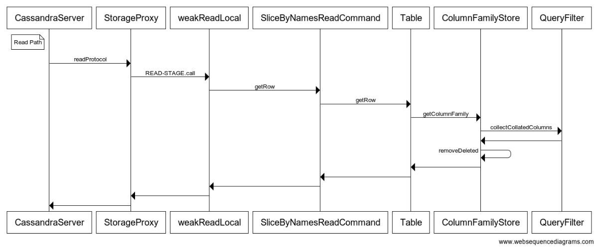
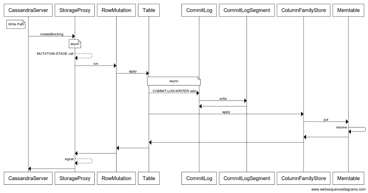
Sequence Diagrams

Sequence diagrams are great at abstracting and visualizing interactions b/w entities. In my case an entity may either be a class, or a STAGE, or a thrift client. Luckily with sequence diagrams you don’t have to be too specific and formal about the kind of entities are used in it, you just represent them all as happy actors (at least, I allow myself to do that, I hope the gods of UML will forgive).

The following diagrams were produced by running Hector’s unit tests and using an embedded cassandra server (single node). The diagrams aren’t generic, they describe only one possible code path while there could be many, but I preferred keeping them as simple as possible even in the cost of small inaccuracies.

I used a simple online sequence diagram editor at http://www.websequencediagrams.com to generate them.

Read Path

Write Path

Table is a Keyspace

One final note: As user of cassandra I use the terms Keyspace, ColumnFamily, Column etc. However, the codebase is packed with the term Table. What are Tables?… As it turns out, a Table is actually a Keyspace… just keep this in mind, that’s all.

Learning the codebase was a large and satisfying task, I hope this writing helps you get up and running as well.

SOCC Keynote Address: Evolution and Future Directions of Large-Scale Storage and Computation Systems at Google

SOCC Keynote Address: Evolution and Future Directions of Large-Scale Storage and Computation Systems at Google

SOCC Keynote Address: Building Facebook: Performance at Massive Scale

SOCC Keynote Address: Building Facebook: Performance at Massive Scale

The Common Principles Behind the NOSQL Alternatives

The Common Principles Behind the NOSQL Alternatives

A few weeks ago, I wrote a post describing the drive behind the demand for a new form of database alternatives, often referred to as NOSQL. A few weeks ago during my Qcon presentation, I went through the patterns of building a scalable twitter application, and obviously one of the interesting challenges that we discussed is the database scalability challenge. To answer that question I tried to draw the common pattern behind the various NOSQL alternatives, and show how they address the database scalability challenge. In this post I'll try to outline these common principles. 

The Common Principles Behind the NOSQL Alternatives

Assume that Failure is Inevitable

Unlike the current approach where we try to prevent failure from happening through expensive HW, NOSQL alternatives were built with the assumption that disks, machines, and networks fail. We need to assume that we can’t prevent these failures, and instead, design our system to cope with these failures even under extreme scenarios.  Amazon S3 is a good example in that regard. You can find a more detailed description in my recent post Why Existing Databases (RAC) are So Breakable!.  There I outlined some of the lessons on how to architect for failures, from Jason McHugh's presentation. (Jason is a senior engineer at Amazon who works on S3.)

Partition the Data

By partitioning the data, we minimize the impact of a failure, and we distribute the load for both write and read operations. If only one node fails, the data belonging to that node is impacted, but not the entire data store. 

Keep Multiple Replicas of the Same Data

Most of the NOSQL implementations rely on hot-backup copies of the data, to ensure continuous high availability.  Some of the implementations  provide you with a way to control it at the API level, i.e. when you store an object, you can specify how many copies of that data you want to maintain at the granularity of an object level. With GigaSpaces, we are also able to fork a a new replica to an alternate node immediately, and even start a new machine if it is required. This enables us to avoid the need to keep many replicas per node, which reduces the total amount of storage and therefore cost associated with it.
You can also control whether the replication should be synchronous or asynchronous, or a combination of the two. This determines the level of consistency, reliability and performance of your cluster. With synchronous replication, you get guaranteed consistency and availability at the cost of performance (a write operation followed by a read operation is guaranteed to return the same version of the data, even in the case of a failure). The most common configuration with GigaSpaces, is synchronous replication to the backup, and asynchronous to the backend storage.
Dynamic Scaling
In order to handle the continuous growth of data, most NOSQL alternatives provide a way of growing your data cluster, without bringing the cluster down or forcing a complete re-partitioning. One of the known algorithms that is used to deal with this, is called consistent hashing. There are various algorithms implementing consistent hashing.
One algorithm notifies the neighbors of a certain partition, that a node joined or failed. Only those neighbor nodes are impacted by that change, not the entire cluster. There is a protocol to handle the transitioning period while the re-distribution of the data between the existing cluster and the new node takes place.
Another (and significantly simpler) algorithm uses logical partitions. With logical partitions, the number of partitions is fixed, but the distribution of partitions between machines is dynamic. So for example, if you start with two machines and 1000 logical partitions, you have 500 logical partitions per machine. When you add a third machine, you have 333 partitions per machine. Since logical partitions are lightweight (they are basically a hash table in-memory), it is fairly easy to distribute them.
The advantage of the second approach is that it is fairly predictable and consistent, whereas with the consistent hashing approach, the distribution between partitions may not be even, and the transition period when a new node joins the network can take longer. A user may also get an exception if the data that he is looking for is under transition. The downside of the logical partitions approach, is that the scalability is limited to the number of logical partitions.
For more details in that regard, I recommend reading Ricky Ho's  post entitled NOSQL Patterns.

Query Support

This is an area where there is a fairly substantial difference between the various implementations.The common denominator is a key/value matching, as in a hash table. Some implementations provide more advanced query support, such as the document-oriented approach, where data is stored as blobs, with an associated list of key/value attributes. In this model you get a schema-less storage that makes it easy to add/remove attributes from your documents, without going through schema evolution etc. With GigaSpaces we support a large portion of SQL. If the SQL query doesn’t point to a specific key, the query is mapped to a parallel query to all nodes, and aggregated at the client side. All this happens behind the scene and doesn’t involve user code.

Use Map/Reduce to Handle Aggregation

Map/Reduce is a model that is often used to perform complex analytics, that are often associated with Hadoop. Having said that, it is important to note that map/reduce is often referred to as a pattern for parallel aggregated queries. Most of the NOSQL alternatives do not provide built-in support for map/reduce, and require an external framework to handle these kind of queries. With GigaSpaces, we support map/reduce implicitly as part of our SQL query support, as well as explicitly through an API that is called executors. With this model, you can send the code to where the data is, and execute the complex query directly on that node.
For more details in that regard, I recommend reading Ricky Ho's post entitled Query Processing for NOSQL DB.

Disk-Based vs. In-Memory Implementation

NOSQL alternatives are available as a file-based approach, or as an in-memory-based approach. Some provide a hybrid model that combines memory and disk for overflow. The main difference between the two approaches comes down mostly to cost/GB of data and read/write performance.
An analysis done recently by Stanford University, called “The Case for RAMCloud” provides an interesting comparison between the disk and memory-based approaches, in terms of cost performance. In general, it shows that cost is also a function of performance. For low performance, the cost of the disk is significantly lower the RAM-based approach, and with higher performance requirements, the RAM becomes significantly cheaper.

The most obvious drawbacks of RAMClouds are high cost per bit and high energy usage per bit. For both of these metrics RAMCloud storage will be 50-100x worse than a pure disk-based system and 5-10x worse than a storage system based on flash memory (see [1] for sample configurations and metrics). A RAMCloud system will also require more floor space in a datacenter than a system based on disk or flash memory. Thus, if an application needs to store a large amount of data inexpensively and has a relatively low access rate, RAMCloud is not the best solution.
However, RAMClouds become much more attractive for applications with high throughput requirements. When measured in terms of cost per operation or energy per operation, RAMClouds are 100-1000x more efficient than disk-based systems and 5-10x more efficient than systems based on flash memory. Thus for systems with high throughput requirements a RAM-Cloud can provide not just high performance but also energy efficiency. It may also be possible to reduce RAMCloud energy usage by taking advantage of the low-power mode offered by DRAM chips, particularly during periods of low activity.  In addition to these disadvantages, some of RAM-Cloud's advantages will be lost for applications that require data replication across datacenters. In such environments the latency of updates will be dominated by speed-of-light delays between datacenters, so RAM-Clouds will have little or no latency advantage. In addition, cross-datacenter replication makes it harder for RAMClouds to achieve stronger consistency as described in Section 4.5. However, RAMClouds can still offer exceptionally low latency for reads even with cross-datacenter replication.

Is it Just Hype?

One of the most common questions that I get this days is: “Is all this NOSQL just hype?”, or “Is it going to replace current databases?"
My answer to these questions is that the NOSQL alternatives didn’t really start today. Many of the known NOSQL alternatives have existed for more than a decade, with lots of successful references and deployments. I believe that there are several reasons why this model has become more popular today. This first is related to the fact that what used to be a niche problem that only a few fairly high-end organizations faced, became much more common with the introduction of social networking and cloud computing. Secondly, there was the realization that many of the current approaches could not scale to meet demand. Furthermore, cost pressure also forced many organizations to look at more cost-effective alternatives, and with that came research that showed that distributed storage based on commodity hardware can be even more reliable then many of the existing high end databases. (You can read more on that here.) All of this led to a demand for a cost effective “scale-first database”. I quote James Hamilton, Vice President and Distinguished Engineer on the AWS team, from one of his articles One Size Does Not Fit All:  

“Scale-first applications are those that absolutely must scale without bound and being able to do this without restriction is much more important than more features. These applications are exemplified by very high scale web sites such as Facebook, MySpace, Gmail, Yahoo, and Amazon.com. Some of these sites actually do make use of relational databases but many do not. The common theme across all of these services is that scale is more important than features and none of them could possibly run on a single RDBMS”

So to sum up – I think that what we are seeing is more of a realization that existing SQL database alternatives are probably not going away any time soon, but at the same time they can’t solve all the problems of the world. Interestingly enough the term NOSQL has now been changed to Not Only SQL, to represent that line of thought.

WTF is Elastic Data Grid? (By Example)

WTF is Elastic Data Grid? (By Example)

Forrester released their new wave report:  The Forrester Wave™: Elastic Caching Platforms, Q2 2010 where they listed GigaSpaces, IBM, Oracle, and Terracotta as leading vendors in the field. In this post I'd like to take some time to explain what some of these terms mean, and why they’re important to you. I’ll start with a definition of Elastic Data Grid (Elastic Caching), how it is different then other caching and NoSQL alternatives, and more importantly -- I'll illustrate how it works through some real code examples.
Let’s start…

Elastic Data Grid (Caching) Platform Defined

Software infrastructure that provides application developers with data caching and code execution services that are distributed across two or more server nodes that 1) consistently perform as volumes grow; 2) can be scaled without downtime; and 3) provide a range of fault-tolerance levels.
Source: Forrester

I personally feel more comfortable with the term Data Grid then term Cache, because Data Grid represents the fact that it's more then a passive data service, but rather one that was designed to execute code. Note that I use the term Elastic Data Grid (Cache) throughout this post instead of just Elastic Cache.

Local Cache, Distributed Cache, and Elastic Data Grid (Cache)

Mike Gualtieri  Forrester Senior Analyst provides good coverage on this topic in two posts. In the first one, titled Fast Access To Data Is The Primary Purpose Of Caching, he explains the difference between local cache (a cache that lives within your application process), distributed cache (remote data that runs on multiple servers (from 2 up to 1000s)), and elastic cache (a distributed cache that can scale on demand).

It is important to note that most Data Grids support multiple cache topologies that include local caches in conjunction with distributed caches. The use of a local cache as a front end to a distributed cache enables you to reduce the number of remote calls in scenarios where you access the same data frequently. In GigaSpaces these components are referred to as LocalCache or LocalView.

Elastic Data Grid and NoSQL

Mike also provides a good description covering the difference between Elastic Data Grid (Cache) and NoSQL alternatives in his second post on this topic, The NoSQL Movement Is Gaining Momentum, But What The Heck Is It? 

Ultimately  the real difference between NoSQL and elastic caching now may be in-memory versus persistent storage on disk.

You can also find more on this in my recent post on this subject: The Common Principles Behind the NOSQL Alternatives

The main difference between the two approaches comes down mostly to cost/GB of data and read/write performance.
…
An analysis done recently by Stanford University, called “The Case for RAMCloud” provides an interesting comparison between the disk and memory-based approaches, in terms of cost performance. In general, it shows that cost is also a function of performance. For low performance, the cost of the disk is significantly lower then RAM-based approach, and with higher performance requirements, the RAM becomes x100 to x1000 times cheaper then regular disk.

The Elastic Data Grid as a Component of Elastic Middleware

In my opinion, an Elastic Data Grid is only one component in a much broader category that applies to all middleware services, for example: Amazon SimpleDB, SQS, MapReduce (Messaging, Data, Processing). The main difference between this sort of middleware and traditional middleware is that the entire deployment and production complexity is curved out by the service provider. Next-generation Elastic Middleware should follow the same line of thought. For this reason, I think that the Forester definition of the Elastic Data Grid (Caching) category should also include attributes such as On-Demand and Multi-tenancy as I describe below:

• On-demand -– With Elastic Data Grid you don’t need to go through a manual process of installing and setting up the services cluster before you use it. Instead, the service is created by an API call. The actual physical resources are allocated based on required SLA (provided by the user) such as Capacity-Range, Scaling threshold, etc. It is the responsibility of the middleware service to manage the provisioning and allocation of those resources.
• Multi-tenancy -- Elastic Data Grid is built provides built in support  multi-tenancy. Different users can have their own data-grid reference while at the same time the data-grid share the resources amongst themselves. Users that want to share the same data-grid instance without sharing the data can also do that through a specialized content based security authorization.
• Auto-scaling -– Users of the elastic data grid need to be able to grow the capacity of the data grid in an on-demand basis, at the same time the elastic data-grid should automatically scale-down when the resources are not needed anymore.
• Always-on – In an event of a failure the elastic data-grid should handle the failure implicitly and provision new alternate resources if needed while the application is still running.

Elastic Data Grid by Example (Using GigaSpaces)

To illustrate how these characteristics works in practice, I'll use the new GigaSpaces Elastic Middleware introduced in our latest product release.

On-Demand

As with the cloud –- when we want to use a service like SimpleDB or any other service we don’t set up an entire cluster ourselves. We expect that the service will be there when we call it. Let’s see how that works.

Step 1 -– Create your own cloud

This is a one-time setup for all your users. To create your own cloud with GigaSpaces all you need to do is make sure that a GigaSpaces agent runs in each machine that belongs to the cloud. The agent is a lightweight process that enables interaction with the machine and execute provisioning commands when needed. The following snippet shows how to start the Elastic Middleware manager and agent. In our particular case, we would start a single manager for the entire cluster and an agent per machine. If you happen to use Virtual Machine you can bundle the agent with each VM in exactly the same way as you would do with regular machines. The snippet below shows the agent command would look like:

>gs-agent gsa.global.esm 1 gsa.gsc 0

What this command does is start an agent with one Elastic Manager. Note that the use of the word global means that the number of Elastic Manager (ESM) instances refers to the entire cluster and not to a particular machine. The agents will use an internal election mechanism to make sure that in each point in time there would be a single manager instance available. If the manager failed a new one will be launched automatically on one of the other agent machines.

Step 2 --  Start the Elastic Data Grid On-Demand

In this step we write a simple Java client that calls the elastic middleware and requests a data-grid service with 1G at minimum and up to 2G (I used these numbers just an illustration that works in a single machine; in a real-life scenario we would expect 10-100G per data-grid).

ProcessingUnit pu = esm.deploy( new ElasticDataGridDeployment("mygrid")
 .capacity("1G", "2G")
 .highlyAvailable(false)
 .publicDeploymentIsolation()
 .maximumJavaHeapSize("250m")
 .initialJavaHeapSize("250m"));

Value Descriptions

• Capacity -– "Minimum", "Maximum" memory to be provisioned for the entire cluster. In cases where highlyAvailable is set to true, the Capacity value should take into account the double capacity required for the backups. In our case that means that setting 1G capacity with highAvliabilty will translate to 512m for data and 512m for backup. Note also that the capacity number defines the capacity for the entire data-grid cluster and not just a single instance. The difference between the Min-Max will determine the level of elasticity that we expect for our deployment.
• High Availability -– When set to true, the elastic manager will provision a backup instance per partition. It will ensure that primary and backup instances wouldn’t run on the same machine. (Note that if you're running a single machine you should turn this argument to false, as otherwise the provisioning will wait infinitely until a backup machine will become available).
• Public Deployment/Isolation –- This is basically one of three isolation/multi-tenancy modes that you can choose for your deployment. The default is dedicatedDeploymentIsolation which means that only one deployment can run on the same machine. In this case we chose public isolation which means that different users share the same machine for deploying multiple data-grid instances.
• Maximum/Initial Heap Size -– This argument defines the capacity per deployment container. The value will be translated into the –Xms, –Xmx JVM argument for each container process.

Using the data grid

Once we have a reference to the data-grid processing unit, we can start and use it.

The next snippet shows how we can write 1000 instances of a a simple Data POJO.

The first step is to get the remote reference of GigaSpace from our deployment.

System.out.println("Waiting for data grid deployment completion ..");
Space space = pu.waitForSpace();
space.waitFor(space.getTotalNumberOfInstances());
GigaSpace gigaSpace = space.getGigaSpace();

Note for the use of waitFor(..) method. The first call waits until the first instance of the space has been deployed. The second call space.waitFor(space.getTotalNumberOfInstances()) waits until the entire cluster has been provisioned successfully.

//Write some data... 

System.out.println("Writing 1000 objects");
for (long i=0;i<1000;i++)
{
 gigaSpace.write(new Data(i,"message" + i));
} 

And here is the Data object for our simple test..

@SpaceClass
public class Data implements Serializable {

 private Long id;
 private String data;
 
 
 public Data(long id, String data) {
 this.id = id;
 this.data = data;
 }

 @SpaceRouting
 @SpaceId
 public Long getId() {
 return id;
 }

 .... setId(), setData(), getData() should appear here.. 
}

Note for the use of @SpaceRouting annotation. Space routing is used to set the routing index, or in other words, it marks the key that determines which target partition this instance should belong to. @SpaceId determines the unique identifier for this instance.

Step 3 -- Give It a Go

Now that we have our cloud running (Step 1) and the client application ready, we're ready to try out our application. All we need to do is run our client application and verify that it works.

If everything works, we should get the following output:

Deploying Data Grid..
Log file: D:\GigaSpaces\gigaspaces-xap-premium-7.1.1-rc…
Waiting for data grid deployment completion ..
Writing 1000 objects
Done!

Now, if we try to run the same application again we would see that it runs much faster. The reason is simply because in the first run we also provisioned our data grid, while in the second run the elastic middleware skipped the deployment step as it already found the data-grid services instance running.

Monitoring and Troubleshooting

To understand what happened behind the scenes we need to familiarize ourselves with the GigaSpaces monitoring tool.

You can use the gs-ui utility located in the GigaSpaces bin directory to monitor the deployment at runtime.

  

You can look at the ESM (Elastic Service Manager) view to see the provisioning and scaling event. You can also view the Agent (GSA) view to see the actual Java command that is passed to the agent to launch new containers. There are plenty of other views and options that will enable you to view the actual data as well as the provisioning steps.

 Understanding the Cluster Sizing

In a cloud environment we normally wouldn't care too much how our service gets provisioned, in this case we would need to better understand how the provisioning algorithm works as we are going to be the owner of both the application and our own little cloud.    

The initial provisioning will fork number of machines/processes based on the following inputs:

- Minimum capacity requested by the user

- JVM capacity per container

- Actual amount of memory available per machine

• Number of partitions: The number of partitions is calculated as follows: With High Availability set to false, Max Capacity/Max Heap Size in our case would be 2G/250m = 8 partitions. With High Availability set to true that would be 4 partitions and 4 backup (1 per partition).
• Number of JVM Containers: In our example the minimum capacity is set to 1G where the capacity per deployment unit is set to 250m. This means that we need a minimum of 4 JVM containers. If we set High Availability to true we would need the same number of containers, but would be able to host only 512m of data, because the other 512m would serve as backup.
• Number of machines: The initial number of machines is a factor of minimum capacity requirements and the actual memory available in each machine. In our example we deliberately chose numbers that fit into a single small machine. If the heap size per JVM container is smaller than the machine available heap size, the Elastic Manager will first try to host more containers to maximize the utilization per machine before it calls for a new machine.

Indeed, if we look at at the deployment view of the gs-ui, we see that in the given case there are currently 8 partitioned being provisioned.

 

 If we examine the host view we see that there are indeed 4 JVM containers being provisioned as expected for the initial deployment.

 

Multi-Tenancy/AutoScaling, Always-On

Elastic middleware supports multi-tenancy and auto-scaling, and it will also keep our data-grid service always-on in case of failure. I've already covered in greater detail how multi-tenancy works here, as well as how high availability works, not just in a local environment but across a disaster recovery site as described here. That said, trying out these features in the context of this example shouldn’t be that hard. You are welcome to play with the isolation argument (Private, Public, Shared), deploy multiple data-grids in the same environment and see what happens. You can also try and break the machines and containers and see how the system heals itself while keeping your application running. You can also launch new containers explicitly (right-click the agent in the management console) or just start a new machine and see how the system scales-out on-demand.

Scaling Down

One thing that is worth emphasizing is how the system scales-down (not just auto-scale). The simplest way to experience how this feature works is to un-deploy our entire data-grid, which you can do by simply calling the undeploy() method:

pu.undeploy();

Another option would from the Administration console: Select the deployment tab and un-deploy the data-grid service from the console.
Now watch what happens to our data-grid instances -- but not only to the data-grid instances but to our containers (processes) as well. Let me explain:
When we un-deploy the data-grid the first thing that happens is that the partitions (the actual data content) get un-deployed freeing the memory within the hosting container. Another thing that happens in the background is that the Elastic Manager notices that we no longer need to run those container processes, and is begins freeing up our cloud environment from those processes automatically… You can watch the ESM logs as this happens.

What’s Next?

Mike includes a roadmap for Elastic Data Grid (Caching) as illustrated in the diagram below.

Since the report was compiled (the report was based on cutoff date of last year) we've already developed a fairly enhanced version of the Elastic Data Grid (Caching) platform. Towards our 8.0 release we’ll have full support for complete application deployment in that same model through the support of a processing unit. In this model you basically deploy an application partition in exactly the same way that you would have deployed a data-grid instance. This will enable us to reuse the same multi-tenancy, auto-scaling and self-healing abstraction that we use for the data-grid for our entire application -- in the exact same way.

Note that current and earlier version of GigaSpaces XAP already support full elastic application and data grid deployment through the SerivceGrid. The Elastic Middleware provides a much higher level of abstraction that makes elastic deployment much simpler to use and much closer to the next-generation data center/Cloud vision.

Give it a try

As noted earlier the example in this post is based on GigaSpaces. To try out the demo you’ll need to download the latest version of GigaSpaces 7.1.1 and follow the instructions above.

Email this

SOCC 2010 updates

SOCC 2010 updates: "

Just came back from the 1st ACM Symposium on Cloud Computing at Indianapolis. The conference is collocated with Sigmod and lasts a day and half. A total of 7 people from LinkedIn were at SOCC and the blog below reflects the notes that we took collectively. There were three keynote speeches, all of which are excellent (the slides will be made available at the conference website).

1. Keynote by Jeff Dean from Google:

• Google already started using flash disks in their clusters.


• Bigtable : It now only runs as a service within google (i.e., one doesn’t install Bigtable himself any more); Each SSTable is validated against the checksum immediately after it’s written, which helps detecting corruption early. This catches 1 corruption/5.4PB data; A coprocessor daemon runs on each tablet and it splits as a tablet gets split. This is used to do some processing on a set of rows and seems to me like a low-overhead MapReduce job since there is no overhead in starting the mappers and reducers.


• Google is working on Spanner, a virtualized storage service across data centers. Didn’t get too much details. The key point seems to be the capability of moving storage across data centers.


• A few key design patterns that worked well in google’s infrastructure: (1) 1 master/1000 workers, simplified design; (2) canary requests: to void an unknown type of request that brings down every worker, first send the request to 1 worker. If successful, send it to everyone; (3) distributing requests through a tree of nodes, instead of direct broadcasting; (4) backup requests to improve the performance of stragglers; (5) multiple small units per machine for better load balancing (don’t need to split a unit and move each unit as a whole); (6) range partitioning instead of hash

2. Keynote by Jason Sobel from Facebook:

• Facebook has 8 data centers.


• Core infrastructure based on sharded MySQL. The biggest pain is that it’s hard to do logical migration (need to split a database). The solution is to over-partition and have multiple databases per node and only move a whole database (similar to the design pattern used at Google). They find that a 3-to-1 file size/RAM ratio ideal for MySQL (with innodb). If the ratio is larger, MySQL’s performance drops significantly. No distributed transactions across partitions. Multi-node updates (e.g., two people becoming friends) are delivered with best effort.


• Heavy use of memcache. Maintain multiple replicas. Want to solve the problem of double caching between memcache and MySQL (the problem is that you can’t take away too much memory from MySQL even though MySQL mostly handles the write load). Memcache is partitioned differently from MySQL. That way, if a memcache server goes down, the read requests on that server are spread across on all MySQL shards.


• Facebook is building FB object/association and a system called TAO on top of memcache. TAO is API-aware and supports write-through on updates (instead of an invalidation followed by a read).


• Facebook has several specialized services: search, ads, PYMK, and multifeed. It uses the search engine to serve complex “search-like” queries over structured data.


• Facebook is building Unicorn. Seems like an event publishing system. Today, it receives batch updates from Hive. It’s moving towards more real-time by taking SQL updates and apply them directly in Unicorn.

3. Keynote by Rob Woollen from SalesForce:

• Most amazing thing to me: there are 4000 people at SalesForce and only 200 of them are engineers (the rest are sales and marketing people).


• It’s using Resin App Server, Lucene, and (only) an 8-way Oracle RAC.


• Dell and Harah’s are among the big customers


• It uses Apex Governor for service protection to prevent a particular tenant from using too much resource. Apex limits things like heap and stack size.


• Flex schema: everything varchar; separate tables for accelerator (indexes), with data types.


• It serves both OLTP and reporting on the same database.


• It uses Ominiscent tracing for debugging : collects log on an operational system so that one can debug locally.


• It uses Chatter for real-time collaboration.

The papers are kind of mixed, likely because this is the very first symposium and nobody knows exactly what kind of papers really fit in. First of all, there are a bunch of papers on MapReduce related stuff.

• Comet: Batched Stream Processing for Data Intensive Distributed Computing. This paper is about sharing work through multi-query optimization. For example, if you schedule a weekly job and a daily job on the same data. The weekly results can be derived from the daily jobs. How to share and what to share is determined through static analysis at a planning phase. The system is built on top of Microsoft’s Dryad.


• Stateful Bulk Processing for Incremental AnalyticsStateful Bulk Processing for Incremental Analytics. The motivating example is how to do incremental crawling.


• Towards Automatic Optimization of MapReduce Programs. This is a position paper and it argues that many database query optimization techniques (both static and dynamic) can be applied to MapReduce. Actually, some of those optimizations have already been applied in systems like Scope.


• Nephele/PACTs: A Programming Model and Execution Framework for Web-Scale Analytical Processing. This is an alternative parallel computing engine to MapReduce. It offers many operators (e.g., joins, filter, aggregation) to construct a data flow, instead of just a map and a reduce operator.

There are several papers related to key-value stores (aka NoSQL databases).

• The Case for PIQL: A Performance Insightful Query Language. It describes a declarative query language for querying key-value stores. The system automatically maintains and selects secondary indexes.


• Benchmarking Cloud Serving Systems with YCSB. It’s a benchmark for comparing various key-value stores (e.g., HBase, Cassandra, sharded MySQL and Pnuts). The benchmark currently focuses on performance comparison.


• G-Store: A Scalable Data Store for Transactional Multi Key Access in the Cloud. This paper adds multi-row transaction support on top of a key-value store that only supports single-row transactions. The approach is similar to Google’s Megastore. The prototype is built on top of HBase, an open source implementation of Bigtable.

Some other papers that I took notes of.

• An Operating System for Multicore and Clouds: Mechanisms and Implementation. This is a paper from MIT on building a virtual Cloud OS (called fos) across multiple cores and multiple machines. This are definitely challenges in how to hide the latency across machines.


• Hermes: Clustering Users in Large-Scale E-Mail Services. This is a paper about clustering users based on their email exchanges. The motivating application is to save space by avoiding storing duplicated messages collocated on the same partition of the backend email server.


• Automated Software Testing as a Service. It’s about using cloud for testing software.

"

How scalable could be a cPanel Hosting service?

How scalable could be a cPanel Hosting service?: "Scalability is one of the important words in the web hosting industry. It is more important than the buzz word 'cloud'. Anyone knows what scalability means, but a very few share the same definition of 'Cloud'. The purpose of this article is to present a hosting service platform which is both scalable and is 'cloud' at the same time.

"

InfoQ: Scale at Facebook

InfoQ: Scale at Facebook

Comparing Document Databases to Key-Value Stores

Comparing Document Databases to Key-Value Stores: "

Oren Eini has an interesting ☞ post emphasizing the main differences between document databases (f.e. CouchDB, MongoDB, etc.) and key-value stores (f.e. Redis, Project Voldemort, Tokyo Cabinet):

The major benefit of using a document database comes from the fact that while it has all the benefits of a key/value store, you aren’t limited to just querying by key.

One of the main advantages of data transparency (as opposed to opaque data) is that the engine will be able to perform additional work without having to translate the data into an intermediary or a format that it understands. Querying by non primary key is such an example. The various document stores provide different implementation flavors depending on index creation time, index update strategy, etc. Oren goes on and covers the query behavior for CouchDB, Raven and MongoDB:

In the first case (nb indexes prepared ahead of time), you define an indexing function (in Raven’s case, a Linq query, in CouchDB case, a JavaScript function) and the server will run it to prepare the results, once the results are prepared, they can be served to the client with minimal computation. CouchDB and Raven differs in the method they use to update those indexes, Raven will update the index immediately on document change, and queries to indexes will never wait. […] With CouchDB, a view is updated at view query time, which may lead to a long wait time on the first time a view is accessed if there were a lot of changes in the meanwhile. […]

Note that in both CouchDB and Raven’s cases, indexes do not affect write speed, since in both cases this is done at a background task.

MongoDB, on the other hand, allows ad-hoc querying, and relies on indexes defined on the document values to help it achieve reasonable performance when the data size grows large enough. MongoDB’s indexes behave in much the same way RDBMS indexes behave, that is, they are updated as part or the insert process, so large number of indexes is going to affect write performance.

Another good resource explaining the differences between MongoDB and CouchDB queries is Rick Osbourne’s ☞ article.

After RavenDB made his appearance in the NoSQL space we’ll probably have to compare it to the existing CouchDB and MongoDB features.

This is not to say that some of this functionality cannot be achieved with pure key-value stores, but these seem to be focused mainly on single/multi key lookups and most probably you’ll have to build this additional layer by yourself.

"